Today I am writing about a free and open source software which is very efficient in calculation and data processing. Scilab is cross platform numerical computing package. It is available in Windows and Linux both. You can use it as open source alternative to MATLAB. If you are a student then you will find it more useful as dont have to spend any bucks for getting the software. This software is having syntax familiar to MATLAB. So iff you are familiar to MATLAB syntax you can easily work with Scilab and if you are not well familiar then this article is for you.
You can download the software from the Home page of Scilab. For Windows platform it is in executable binary setup form. For other OS it is in compressed setup form. If you are using Ubuntu Linux you can install it from package manager. After install it is ready to be used out of box.
So lets run some of basic commands on it.
Lets create a matrix. Commands and outputs are given in evenly spaced font.
-–>mat = [1,2,3;4,5,6;7,8,9]
mat  =
    1.    2.    3.
    4.    5.    6.
    7.    8.    9.
We created a 3X3 matrix using above command. Now lets create transform of our recently created matrix.
-–>trans_mat = mat’
trans_mat  =
    1.    4.    7.
    2.    5.    8.
    3.    6.    9.
So we got transform of matrix stored in trans_mat variable. We can also perform other operations on our matrix. For example inv(mat) will find inverse of matrix if it is not singular.
Scilab has wide variety of inbuilt functions. It can plot the results. You can format your plotted results as per your requirements. Next we can take example of plotting a sine wave. Enter the following commands in your Scilab terminal.
t = -2*%pi:0.01:2*%pi;
y = sin(t);
plot(t,y);
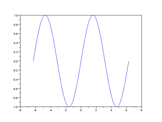
What you will get after executing the above commands will be a graphical window with following graph.

This is our plotted sine wave. We can modify the appearance of this wave in several forms. Type following command in terminal window.
plot(t,y, 'r')
What do you see? Your plot has changed to red color. This can be very handy while you are plotting several graphs on same plot. Want to see it in action. Run the following set of commands.
t = -2*%pi:0.01:2*%pi;
y = sin(t);
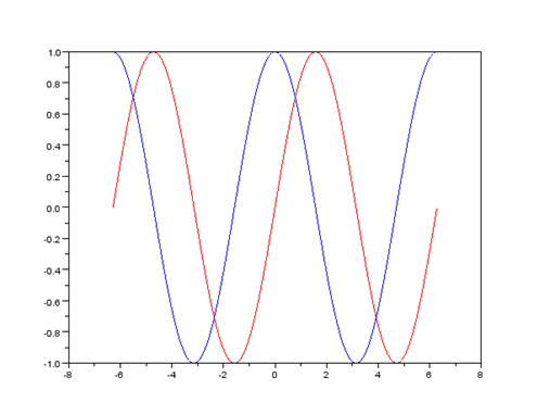
plot(t,sin(t),’r',t,cos(t),’b')
And here is output.

So here are plots for sin(t) and cos(t). We have assigned them different colors while plotting so we can easily recognize our plot. But how about putting a legend. Legend make our graphs more readable to end user. So put a legend using next command.
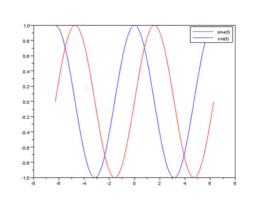
legend("sine(t)", "cos(t)")
You will see your graph will have legend as shown in next figure.

So here is our final readable output. We can create Bode plot and other plots also using Scilab. I think till now you are ready to go with the tool. We will be using this tool ahead in our coming tutorials.